SQL Table and Field Extraction

 Post Index

2023-12-02

SQL Table and Field Extraction

Analyzing and Parsing SQL

How to design, analyze and explore 

for 

the SQL parsing and extraction

SQL is very common in the realm of the data world.  In every second, there are a huge number of SQL queries being executed to perform operations in databases.  It is all over the world, both externally and internally in organizations.  There are many data roles and positions are requiring SQL skills to support all kinds of data applications and analytics.  Nonetheless, the overwhelming demand leads to a common question to understand what data have been used.  A lot of organizations are looking for solutions on how to understand the data cycles, the data lineage and the data governance.  Unfortunately, there is no handy tool available.  In particular, parsing the SQL query and extracting the underlying tables and fields are also unavailable.

For this question, I have been asked for a solution quite a few times.  The intuition is that even there is a way to do, it would not be perfect.  Apparently, it is time-consuming and required plenty of tests and experiments.  In terms of the overall priority in organizations, it is 100% not in the top priority list.  Thus, even there is interest, there is no one trying to work out in this area (maybe there is, ping me and let me know).

Nonetheless, I think it is good to try this out.  One of the reasons is that this can be a good exercise to practice different skills like design skill, analysis skill, problem solving skills, coding skill, etc.  Another reason is that it is possible to be a core component in the future of data realm (perhaps GenAI can do later?).  I am hoping that it can benefit to the people looking for the same solution.

As a result, in this article, I am going to provide the details on how this question is answered.  I will try best to provide my step by step thinking and analysis for reference so that you would be able to pick up the skills I did.  Or share me something new based on what I have done.

OK.  Let's start.

* the tables in the article also refers to tables or views.

Overview of SQL Query

Let's take an example of a SQL query that I obtained from the web.

SELECT
  DATE_FORMAT(co.order_date, '%Y-%m') AS order_month,
  DATE_FORMAT(co.order_date, '%Y-%m-%d') AS order_day,
  COUNT(DISTINCT co.order_id) AS num_orders,
  COUNT(ol.book_id) AS num_books,
  SUM(ol.price) AS total_price,
  SUM(COUNT(ol.book_id)) OVER (
  PARTITION BY DATE_FORMAT(co.order_date, '%Y-%m')
    ORDER BY DATE_FORMAT(co.order_date, '%Y-%m-%d')
  ) AS running_total_num_books
FROM cust_order co
INNER JOIN order_line ol ON co.order_id = ol.order_id
GROUP BY 
  DATE_FORMAT(co.order_date, '%Y-%m'),
  DATE_FORMAT(co.order_date, '%Y-%m-%d')
ORDER BY co.order_date ASC;

In the SQL query, there are many elements:

1. SQL Clauses, e.g. SELECT, FROM, JOIN, GROUP BY, ORDER BY, etc.
2. Functions, e.g. DATE_FORMAT, SUM and COUNT.
3. Table, e.g. cust_order, order_line
4. Field, order_date, order_id, price, etc.
5. Alias, for table, e.g. co (cust_order), ol (order_line).  For field, e.g. running_total_num_books.
6. Reserved Word, e.g. ASC, INNER, ON, etc.
7. Text, they are enclosed by single quote, e.g. '%Y-%m-%d'.  After the start of single quote, it can be any character until the pair of quote is met.
8. Separator, e.g. commas (,), space ( ), newline (\n), bracket, etc.  I refer them all to symbols.
9. Dot, it is used to separate the server, database, schema, table and field.  Usually, server, database and schema can be omitted

In fact, there are a few other possible elements not showing the example:

1. Comments, it can be either // or /* */ or -- depending on which database and its proprietary syntax.
2.  Double Quote, it is used for explicitly to provide the object name to escape some characters, e.g. "My Column".  Space in it will be treated as a character of the field name.
3.  Asterisk (*), it is a special indicator to get all the fields.
4. Operators, e.g. +, -, *, /, ||, etc.

As you can see, there are a lot of details are conveyed inside the SQL query.  This is my first basic understanding about the SQL query by some known knowledge and observations.  The initial is started by the above.  And later on, if more scenarios come in, it will be enhanced case by case.

Tokenize the SQL Query

After the SQL query overview, next I am thinking to tokenize the SQL query.  It is to construct a way to break the SQL query into tokens.  It is important to be able to identify each component in the SQL before we can analyze and identify the table or field.

However, how to do it?  A straight way from everyone would be using whitespace, i.e. space, new line, tab, etc as a separator to 'chopped' the SQL into pieces.  Then let's have a try.

Based on the example, the below result will be obtained:

1. SELECT
2. 
3. DATE_FORMAT(co.order_date,
4. '%Y-%m')
5. AS
6. order_month,
... ...

Apparently, it is not as our expectation.  However, let's calm down, observe and analyze the results.

1. Whitespace is possibly one of the separators.
2. It looks like symbols can also be a separators.  e.g.  bracket, comma, single quote, etc.
3. The separator (either whitespace or symbol) is right after the end of each token.  

Then, let's revise the separator list as below.

1. \s (whitespace)
2. ,
3. +
4. -
5. *
6. /
7. \
8. (
9. )
10. . (dot)
11. "
12. '
13. = 
14. <
15. >
16. ;

Then, let's re-try the tokenization (this can be achieved by using regex, I will focus on the concept and idea in this article.  If there is a need for more details in the regex, leave me a comment).   So, the tokenized result will be like:

1. SELECT
2. DATE_FORMAT(
4. co
5. .
6. order_date,
7. 
7. '
8. %Y-%m'
9. )
10.
11. AS
11. order_month,
... ...

Thus, each token is now either clean without a suffix symbol or not clean with a suffix symbol.  Thus, it would be possible to further separate the symbol into next row, i.e.:

1. SELECT
2. DATE_FORMAT
3. (
4. co
5. .
6. order_date
7. ,
8. 
9. '
10. %Y-%m
11. '
12. )
13.
14. AS
15. order_month
16. ,
... ...

After these steps, each token now is clean, i.e. either a word or a symbol.  Then next, the tokens are required to be manipulated into SQL unit.


SQL Unit

SQL unit, basically, refers to the unit that is recognized as an human recognizable object (I am not quite sure how to call it and so named it SQL unit).  For example, 'Hello World', the entire 'Hello World' is a SQL unit.  Another example, Field as "Renamed As", "Renamed As" is a SQL unit.  Another example, mySchema.myTable.myField, the entire string is a SQL unit.  From human interpretation, they are a single unit.

The SQL unit is atomic and with unique meaning.  Examples of SQL unit are:

1. string, each single quote pair will be become one SQL unit.
2. multirow comments, everything inside /* */ means to be a SQL unit.
3. double quoted string, each double quote pair will become one SQL unit.  It is similar to single quote.
4. dot, the dot will concatenate the server, database, schema, table and field as a SQL unit.

The pattern in the tokens are therefore analyzed to combine together as SQL unit.  As a result, the below will be obtained:

1. SELECT
2. DATE_FORMAT
3. (
4. co.order_date
5. ,
6. 
7. '%Y-%m'
8. )
9.
10. AS
11. order_month
12. ,
... ...


As can be seen, co.order_date is SQL unit of field,  '%Y-%m' is a string for date formatting, etc.

Up to this moment, the whitespace at beginning and the end is actually redundant because the meaningful whitespace is already included inside the SQL unit.   After trimming (or remove), it will be like:

1. SELECT
2. DATE_FORMAT
3. (
4. co.order_date
5. ,
6. 7. '%Y-%m'
7. )
8. AS
9. order_month
10. ,
... ...



Then next, it is going to identify patterns.  There are a few things can be identified.



Identifying SQL Clause

SQL query has a syntax to follow and the syntax is actually explained by SQL clauses.  For example, Select clause to have all the fields to be extracted from the table/view.   From clause to specify tables/views.  Dependent on which database is used, the clauses might be slightly different.  But in general, the below must be able to be identified.

1. SELECT
2. FROM
3. JOIN (From)
4. ON (From)
5. WHERE
6. GROUP BY
7. ORDER BY 
8. etc

Identifying the SQL clauses can help to distinguish the extracted SQL unit is a table or is a field.  Obviously, table can only be found in FROM Clause and JOIN (From) clause.  Field can be found in all other clauses.

* it should refer to the syntax of the SQL query allowed in the database.

Identifying Subquery

Subquery is inside a SELECT statement, there is another SELECT statement.  It can appear in SELECT clause for scalar output, or in FROM, JOIN (FROM) clause as temporary table result.

Subquery is easy to determine because it must be between a pair of bracket and starts with SELECT, i.e. (SELECT ... ) 

Identifying subquery is important because in terms of table and field extraction from the SQL query, the only focus is the first time of use.  The nested subqueries are usually re-using the extracted fields to continue calculation.  The hierarchical usage will not be a concern.

Based on this, the subquery is required a SubqueryID.  So that the table and field can be matched within the same subquery.  With this concept, it facilitates the matching processes for table and field.  It will discussed later in the article.

Identifying Function

Function is always expressed in the form like function (parameter1, parameter2, ... , parameter n).   It must have a bracket to include a parameter list.  Thus, if bracket is found and it is not a SQL unit of subquery, it must be function.

Function means that it neither table nor field.  Thus, it should be ignored for the extraction.

Identifying Special Patterns

This is very difficult to define them in the first place.   It is required a lot of testing of SQL queries to figure this out.

First example is at time zone.  All three words in this special pattern is not in the reserved word list.  But they are allowed in SQL to specify the timezone.  It can be tracked as a SQL unit.  But no matter what, they are ignored as they are not table or field.

Another example is date component appearing in some of the date functions,  e.g. date_trunc(year, DateField)

Usually, inside the function call, it is either a field, a number or string.  For specific function like date_trunc, date_part, date_dateadd, extract and datediff, these functions will take a parameter call date part to indicate which date component to be used, e.g. year, month, day, etc.  They are neither required to be quoted nor are reserved words.   A special pattern is required to identify this.

* Just take a note that there might be more to be figured out.

Identifying Alias
There are different patterns for alias.  They include:

1. SQLUnit as Alias

It is typical, e.g. field as fieldName or table as tableName.

2. SQLUnit Alias

It is also typical to omit the AS, e.g. field fieldName or table tableName.

3. SQLUnit "Alias" or SQLUnit as "Alias"

It is also typical to define the alias with double quote to escape the special characters, e.g. field "field Name" or table as "table Name".  AS can be optionally be used.

4. With Alias

Alias inside the with clause is having a special syntax that allows multiple queries to be first executed and named aliases.  Then a following query will make use of those temporary results to complete the final the SQL result.

e.g. WITH t1 AS (

SELECT AVG(Sales) AVG_SALES FROM Store_Sales

)

SELECT a1.* FROM Store_Sales a1, t1

WHERE a1.Sales > t1.AVG_SALES;

Instead of specifying the alias at the end, it is specifying the alias at the very beginning.  The example t1 is the alias for the result SELECT AVG(Sales) AVG_SALES FROM Store_Sales.

Therefore, it is possible to know aliases of fields and aliases of tables.

Removing Objects
The original purpose is to find out table and field used in the SQL query.  Thus, it means to remove all other that are not tables nor fields.  They include:

1. Reserved Words
2. Functions
3. Symbols (separators)
4. Comments (single row comment // and multirow comments /* */)
5. String
6. Operators
7. Numeric 
8. Identified Patterns
9. Aliases

Once all the above are identified and removed in the SQL query, the remaining is only table or field.

The removing objects are identified based on regression test.   Once the result is obtained, it is obvious to notice what is further required to remove.  The above list is at least running 10+ times of different queries to identify.

Once the patterns are identified, next is to finalize the table and field discovered.

Matching Table and Field

After tokenization, SQL unit combination and pattern identification, the next will be to match the table and field against the metadata in the database.

For table, it is straightforward to obtain the table from the FROM or JOIN (FROM) clauses.  But for field, it is a bit tricky.

Because of the possible use of asterisk, the only possible way is to to cross check against the database metadata.  Otherwise, it is impossible to know what fields are included.  Also, the field specified in the SQL query is usually without the table prefix.  Unless, there is a full list of metadata to cross check, it is impossible to ensure the field belongs to which table.

To match the field, there are different matching required:

1. Match the exact name (no table prefix)
2. Match with alias
3. Match the Full/Partial FQDN  (database.schema.table.field)

Each FROM clause or JOIN (FROM) clause is specifying the table while the corresponding select clause is specifying the field.  So, each subquery, an SubqueryID has been assigned.  The outmost query is 0.   As a result, the field must come from one of the tables with the same SubqueryID.   Thus, the above 3 matching criteria, either one will ensure a match.

* it is assumed the query is syntactically correct and is executable without error.  Thus, cross-checking with database metadata, the answer is unique.

Matching Asterisk

The match for asterisk is similar to have:

1. Match with alias
2. Match the Full/Partial FQDN

But instead of matching a single field, it is getting all the fields inside the specified table.  If not prefix, it means all fields in the table list.

Conclusion

The purpose of this article is not trying to provide a tool for this purpose but to share the understanding and exploration that have been done such that the mindset of tackling this kind of problems can be understood.  Or if possible, to enable you to think further.

There is an assumption that the SQL query must be syntactically correct and the SQL is runnable.  The extraction is not doing debugging but instead, it is purely pattern recognition.

The method discussed still cannot promise a 100% extraction but to continue for more test cases and patterns to be identified, it will eventually becoming 100% (Also, it depends on which SQL standard is used and it is varied).  But in terms of our own testing, it can tackle majority of the SQL queries.

At the end, I would like to say "practice makes perfect".   Try more and you would learn more.

Thanks for reading.  I hope you enjoy my post.

By the way, share me your thoughts, leave me comments.

Agile Project Management - Requirement Log, Issue Log and Test Log

Post Index

2023-11-18

Agile Project Management

Requirement Log, Issue Log and Test Log

How to use make use of simple Excel log files 

to 

manage data analytic project

With the fast growing world, agile project management is very common nowadays and it has a lot of advantages over waterfall project management, in particular to data analytic project.  One of the apparent reasons is that data analytic project usually involves data exploration and data analysis which is not possible to define all requirements beforehand.  It, in fact, involves a number of try-and-error to understand the relationship of data and try to figure out patterns and methods that are useful for business users to find insights.  To make it simple, it would be easier to understand by the phase "seeing is believing", i.e. creating a mockup dashboard will win over a thousand words to describe the details.  Thus, in agile data analytic project, a number of sprints/cycles is in place to develop, to mockup, to revise, to enhance until the ultimate and desired dashboard is completed.  Unless, there are explicit requirements.  Usually, a time-box approach will be used.  More often, a rough estimation is proposed for initial requirements and based on the development sprints, more in-depth discussion will take place to finalize the dashboard.

However, how to manage the detail and discussion? In this article, I will share how I use the simple documents to keep track the status and details on this kind of agile data analytic project.  The documents include:

• Requirement Log

• Issue Log

• Test Log

These are Excel documents for easy maintenance.  Definitely, the same concepts can be applied into project management application.  It depends on what is available in your organization.

Requirement Log 

Requirement log by its name is to log the requirements.  Its main purpose is to keep track of the discussion of requirements from initial high level discussion to detail on how to implement each charts in the dashboard.  It also includes the data mapping indicating the source table/view and field and description on how to derived new fields.

The requirement logs contains of two sheets:

• Requirement Log - the detail and status of the requirement.

• Screen Capture - to provide screen capture/pictures for requirement.

• # - it is ID of the requirement.

• Log Date - it is the date that the item is logged.

• Raised By - it is who provides the requirement.

• Follow up by - it is who to follow up the implementation of the requirement.

• Last Follow Up Date - when this item has been last updated.

• Priority - the priority to indicate the importance.

• Status - New, In Progress, Pending Confirmation, Completed, etc, i.e. a status that can indicate the situation.

• Description - the details of the requirement.

• Remark - additional information to supplement the item.

• Screen Capture - it is providing a reference number of the screen capture, e.g. #1

To highlight a bit on the description, it is in the format like below:

YYYY-MM-DD (Who logged)

Details

The description is accumulated.  Therefore, whenever, there is an update of the requirement or there is any discussion, it will be logged down in the description.  As a result, there is a very clear trace of the requirements.  And the requirement can be started very high level, e.g. a dashboard for support cases to use major KPI.  And this item can be Closed while it is further broken down into other items to continue the follow-up.  The description can simply reference to the # number to indicate the trace.  It looks simple but it also requires experience to wisely use this requirement log.

For the screen capture, normally, it is very difficult to put this into Excel because when there is a long description, it requires more space and it leads to the misposition of the screen capture and eventually mess up the entire document.  A wiser approach would be freely to put the screen capture into another sheet with a # number.  And when required, it can locate the screen capture.  When you try it out, you will find its beauty.

All items must be completed or closed before it can go into the testing/UAT stage.
In the requirement log, it also contains table and field, derived field as a requirement.  Here, I do not go into details of this as it is quite common to have a list fields to be used and how they will be renamed as business name.  But, it should be emphasized that it can add more sheets as a support of the requirements.  It aims at having a single truth of requirements.

Issue Log

Issue log is very similar to requirement log to have two sheets including issue log and screen capture.  It aims at tracking all the issues arise in the project.  The issue log contains the follow columns:

• # - it is ID of the issue.

• Log Date - it is the date that the issue is logged.

• Raised By - who reports the issue.

• Follow up by - who is following up the issue.

• Last Follow Up Date - when this issue is last followed up.

• Category - which area this issue is belonging to.

• Status - New, In Progress, Resolved, etc, a status to indicate the progress.

• Description - the details of the issue.  It has similar format to requirement log having date, who and details for each follow up.

• Action - what actions have been done to fix the issue.  It has similar format to requirement log having date, who and details for each follow up.

• Screen Capture -  it is providing a reference number of the screen capture, e.g. #1

To reduce the number of document, requirement log and issue log could be combined into a single document for easy management and follow-up.
All items in the issue log are required to be resolved before it can go into testing stage.

Test Log

Test log is also very similar to the requirement log but the details are focusing on the testing issues.  It contains the following columns:

• # - it is ID of the testing issue.

• Log Date - it is the date that the test issue is logged.

• Raised By - it is who finds out the issue.

• Follow up by - it is who to follow up the fix.

• Last Follow Up Date - when this item has been last updated.

• Description - the details of the issue.

• Status - New, In Progress, Pending User Check, Pending Fix, Fixed, etc, i.e. a status that can indicate the situation.

• Screen Capture - it is providing a reference number of the screen capture, e.g. #1

All items in the test log must be completed before it can start the migration process to production.

Conclusion

These three documents including requirement log, issue log and test log can already tackle majority of agile data analytic project.  This simple framework is still required experience on how to write the details in a meaningful way.  One rule of thumb is to bear in mind of MVP, i.e. minimal viable product.  In other words, it should not have redundant details.  All details should be neat and simple.  However, it depends on your understanding and how you can ignore the "noise" and irrelevancy.  I have been using this for a few years and working fine and there are a number of fellow also available to pick this up and continue this kind of neat and MVP approach.  Try this out and see if you can ride on the concepts for your data journey.

I hope you like the sharing.  Thank you for reading!  Drop me a message for discussion.

Masking Data Environment

Post Index

2023-10-07

Synthesize Data Environment

Techniques Sharing

How to use Production Data to Synthesize Sample Data 

for 

Development and Testing

One of the issues in data realm is that there is a lack of development and testing data.  Even though it claims to have testing data available, they are loosely coupled and does not conform to the data integrity.  Using this kind of development and testing data may not cover all scenarios that may happen in production.  And thus, in development and testing, it does not come with the best results.  Even worse, it increases the effort, difficulty, time and cost.

Ideally, the production data is of the best to be used for development and testing but there are many reasons like security, performance, maintenance concerns, etc to hinder this possibility.  In this article, I will try to share some ideas and techniques that might be possible to use production data to generate development and testing data.  The method to be discussed might not be perfect and it still requires more input and enhancements.  The idea, however, is good to be shared and discussed.  Kindly let me know what you think and leave a message for discussion.

Techniques

There are a few techniques to be used including:

• Data Masking
• Data Shuffling
• Randomizing Values

These techniques can be applied individually but to get a better result, a combination of them is required.  Imagine that the production data is the best source for development and testing because it has all actual scenarios captured in the dataset and all columns are with the expected values already.  However, because of the data sensitivity, it is not open to everyone.  Thus, further to image that if the values in the data table are all maintained, the values are just shuffled, masked or randomized, it is a close to the production data.  Although the integrity might not be 100% enforced,  majority of the synthesized data is already possibly enough for development and testing.

Some simple analysis can be performed in each table to see which methodology would be best fit to be used.

Data Masking

Data masking is obviously to mask the data.  To be more specific, it can be achieved in several ways:

• hash function mask (string / integer)
• fixed string/number mask

Hash function mask is to apply a hash function to the values such that a fixed string or fixed number can be generated.  This operation is irreversible, i.e. the hashed value is not able to be generated back to the original value.  Some examples of hash function are SHA1, SHA2, MD5, etc.  Apparently, it is able to "guess" or "deduce" the original values if the provided values can generate the same hash values.  In order to avoid such situation, a fixed constant, current date, can be added to the value for the hash generation.

Fixed string/number mask is to convert the value into a fixed string or number.  If it is too sensitive, it's better just to masked it with ***MASKED DATA*** for example.

Data Shuffling

Data shuffling means that all the values in the column are shuffled. This is good to maintain the general values such as gender (Male, Female), Product, etc.  The shuffled values are still meaningful but they are in another rows.

Data shuffling is also very useful to be applied in the key column.  Thus, the data association will become more random.

Randomizing Values

Randomizing values obviously is to randomize numbers, dates or values.  

For number, it is easy to apply random function.

For date, it is easy to apply random function as well with a start date.  The start date plus the randomized days will become the randomized date.

For values, a list of value should be ready beforehand and the random value will be based on the list.  

Random values are always bounded by a range or a list of values.

More Considerations

In general, there are several kinds of data:

• Key
• Fixed list of data values
• Fixed range of values
• Free Text

Key - if it is not sensitive, shuffling would be enough.  Otherwise, apply data masking and shuffling.  For masking, it is a must to apply a fixed constant or date into the hash function.

Fixed list of data values - shuffling or randomizing would be good choices.

Fixed range of values - randomizing would be good.

Free text - not applicable for the above techniques.  There are more considerations.

The synthesize data is not trying to duplicate the entire production data and convert them into development and testing data.  Only a portion of them can be extracted and applied the above techniques.  And synthesizing the data periodically is good practice to lower the chance the data can be deduced.  

Conclusion

The above techniques are not perfect but it is a starting point to consider how to automate for development and testing data.   One beauty of the above techniques is because of its simplicity.  The idea is not trying re-produce the full set of production data but a portion of them to be enough to facilitate development and testing.  There are possibly plenty of other methods to achieve the same purpose.

Currently, there is also topic on generative AI to generate data for the same purpose.  Perhaps, a combination of the techniques and AI power will be the next phase to move on.

I hope you like the sharing.  Thank you for reading!  Drop me a message for discussion.

QlikView Metadata Extraction

 Post Index

2023-09-30

QlikView Metadata Extraction

Automated Metadata Extraction

How to automate the extraction process

QlikView was a very good product in analytics.  It has been developing so well and now is going to fade out in the market.  QlikView is now having very few updates and minimal support.  A lot of companies are planning to migrate QlikView applications to Qlik Sense applications or other analytic tools like Tableau or PowerBI.

In order to perform the migration, apparently, it is not an apple-to-apple.  No matter on design or the end-to-end data flow, there will be differences.  Thus, to increase the successful conversion, there is a need to extract the metadata in QlikView.  Instead of browsing all details in the QV applications, extracting the metadata will make it easier to understand the applications and design.

This article is going to share the automatic method to extract the metadata.   And I will also share some ideas on how to use this metadata.

QlikView COM API

In QlikView, there are a tool called QlikView COM API.  It is available to be used for automation and macros.  It can also be used in creating standalone Windows applications with its OCX component.  The QlikView COM API reference can be found here.

After downloading and unzip, there is a QVW application to illustrate all the API available.

Important Metadata

In general, two kinds of metadata are required:

1. Layout file

It contains all the QV properties in the application.  Apart from calling API, in fact, this can also be extracted via the front-end (* this will separate all individual components per XML file)

2. Variables

There are plenty of ways to extract variables.  For example, people might write script to get the values of each variables and put into a table, then export the details into csv.  In order to from metadata level, API can be used.

With both the XMLs and variables, it is very easy to trace the expression used in each chart.  And further analysis can be done to review how they can be implemented in other analytic tools.

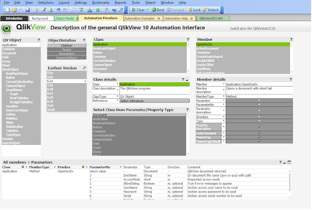
In the QlikView COM API Guide application, there is a sheet named "Automation Members" to review the parameters of each method.

And there is a sheet "Automation Examples" that illustrates an example of the API call.

Using the QlikView COM API

The metadata extraction pseudo steps are described as below.

1. Define the paths, e.g. QV doc path, layout folder path, variables.csv path.

2. Create the QlikView object.

3. Open the QV document.

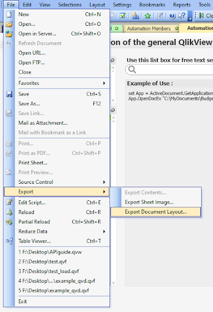
4. Export the layout files.

5. Get the variable list

6. Loop through the variable list and construct a format for csv output

7. Close and clean up the resources.

In order to use the API, VB script can be used.  The complete VB script is as follow.

'Paths

dim qvDocName, layoutFilePath

qvDocName= "D:\qv.qvw"

layoutFilePath= "D:\layout\layout.xml"

variableCSVPath= "D:\variables.csv"

'Create QV object

set qv = CreateObject("QlikTech.QlikView")

'Open QV doc

set qvDoc = qv.OpenDocEx (qvDocName, 2 , false , "" , "", "" , false)

' Export Layout Files

qvDoc.ExportLayoutFile(layoutFilePath)

' For variable CSV output

Set objFSO = CreateObject("Scripting.FileSystemObject")

CONST ForWriting = 2

'Open the CSV file for writing

Set objTextFile = objFSO.OpenTextFile (variableCSVPath, ForWriting, True, -1)

'CSV header line

objTextFile.WriteLine("VariableName|||VariableValue|||RawVariableValue|||")

Set vars = qvDoc.GetVariableDescriptions

for i = 0 to vars.Count - 1

set v = vars.Item(i)

        ' using ||| as delimit will be easier to avoid the newline and quote issues in CSV during read.

        objTextFile.WriteLine(v.Name &" |||")

        objTextFile.WriteLine(qvDoc.GetVariable(v.Name).GetContent.String &" |||")

        objTextFile.WriteLine(v.RawValue &" |||")

next

objTextFile.Close

qvDoc.CloseDoc

qv.Quit

Parsing the XML and Variables

The XML is well formatted and it contains all the properties of all charts, sheets, texts, etc.  To be simple, the most important are charts, dimension and measures.  By extracting these from the XML, it can have a basic ideas of the complexity of the application.

Usually, in the expression, a lot of variables will be used and more often, they are nested.  It is not easy to trace them level by level because there is a lot of back-and-forth to review each step.  In QlikView, dollar sign expansion is used to get the value of the variables.  With this understanding, it is possible to use $(variablesName) as a mapping to match the value from the variable list extracted.   In such a way, the variable used in each chart can be expressed in the most detailed format where all variables are extracted.

Although this cannot resolve dynamic variables, to certain extent, it helps a lot in digesting the information in QV.  This article would not cover the extraction part.  But in case if you think it is interesting, do drop me a message and I will see if a guide can be provided later.

Thank you for reading.  I hope you like the sharing.  Leave me message and let me know what you think.

Analytical Calendar - Technical Discussion

Post Index

How to Use | Analytical Calendar The Story | The Index Page

2023-09-23

Analytical Calendar

Technical Discussion

The technical design in detail

Analytical Calendar is extremely useful to be used in interactive dashboard.  I have shared a number of articles related to this topic and hope that everyone can understand the ease and the difficulty when dealing with date and calendar.  Different people might have different perceptions on how to use date and calendar.  It is impossible to change the mind if it is already becoming a habit or get used into the same regular actions reacting daily.  However, it is worth that you can try and understand further of what Analytical Calendar is and how it can make a difference in your analytic dashboards.

This article focuses on the technical design of analytical calendar and let you understand how it can make your life easier from the development and also from your daily use in analytics.  One of the nice stuff is that the date associations are already built inside the Qlik associative data model.  For developer, you don't need to work out a lot of set analysis to come up with the correct period.  For analyst, you don't need to work have a lot of charts developed and the perspective for period is simplified into analysis and comparison periods.

If you are not familiar with Qlik associative data model, please try to get some understanding in the Qlik website first.  Also if you have forgotten how to use the Analytical Calendar, please review in the previous post.  Or if you have interested in how the analytical calendar comes up, you can click the link at the top to follow the story.

Analytical Calendar Data Model

First, let's look at the data model of the Analytical Calendar.

Analytical Calendar consists of five core tables.  As shown in the above data model diagram, they include:

1. ANALYSIS_CALENDAR

This is the analysis calendar.  It controls the selection of "Date Perspective", "Unique Date" and "Analysis Perspective".  The main purpose of this table is to allow selection of analysis period.

2. %CUSTOM_LINKEDTABLE

It is a linked table to associate the ANALYSIS_CALENDAR to the PERSPECTIVE_CONTROL_CALENDAR.  This table exists because of the need of Custom Unique Date selection as a comparison.  Each analysis period, in fact, is associating a number of available comparisons.

3. PERSPECTIVE_CONTROL_CALENDAR

It controls the "Comparison Perspective" selection and it is also used to associate to the date range required in %DATE_RANGE_LINKEDTABLE.  Each row is associating to a corresponding date range (i.e. %DATE_RANGE_KEY).  This is a very important table because it has all date and calendar information, i.e. ANALYSIS, COMPARISON, CUSTOM.

4. %DATE_RANGE_LINKEDTABLE

It is associated a date range to the dates in the range.

5. DIM_CALENDAR

It is the dimension table of calendar to facilitate all the chart requirements on date and calendar.  It has all combination of date components and the corresponding sequence.

There is a TRANSCATION table that is a dummy fact table for demonstration purpose only.

More on the Technical Design 

There are a couple of "magic" lightened up the Analytical Calendar.

Analysis is a subset of Comparison

If you are small-hearted, you will notice the relationship between analysis and comparison in Analytical Calendar .  To do analysis, you need to select

1. Date Perspective

2. Unique Date

3. Analysis Perspective

To do comparison calendar, you need an additionally Comparison Perspective.  in other word, you must first have the analysis before you can do the comparison.  So, there are tables ANALYSIS_CALENDAR, %CUSTOM_LINKEDTABLE and PERSPECTIVE_CONTROL_CALENDAR in the design to allow each analysis period to associate with all possible comparison periods, either comparison range or Custom Unique Date.

Taking an example of analysis period MONTH, 2023-Mar, YTM.  It is associating with all comparison like 1 year before, 2 years before and so on, and Customer Unique Date like 2023-Jan, 2023-Feb, etc.  This kind of association is built inside the data model.

From another point of view, in term of data-wise, it looks like analysis is a subset of comparison in terms of the required selections.

Generic Keys for Custom Unique Date Association

Interestingly, there is a table called %CUSTOM_LINKEDTABLE.  Originally, the ANALYSIS_CALENDAR can directly associated to PERSPECTIVE_CONTROL_CALENDAR.  In order to allow Custom Unique Date selections, this table is using the concept of generic key.  Thus, all Custom Unique Date can be associated to any analysis period in ANALYSIS_CALENDAR.

If Custom Unique Date is not required, this table is apparently not required.

Magic %CONTROL_PERSPECTIVE

The %CONTROL_PERSPECTIVE is, indeed, the main control of which period to be applied.  If no value is selected in this field, it means all analysis and all comparison.  If "ANALYSIS" is selected, it means to enable analysis perspective but apparently, "Comparison Perspective" must be ignored, i.e. {<%CONTROL_PERSPECTIVE={'ANALYSIS'}, "Comparison Perspective"=>}.  On the other hand, to enable comparison, it needs to ignore ANALYSIS, i.e. {<%CONTROL_PERSPECTIVE-={'ANALYSIS'}>}.  Regarding to the selection in "Comparison Perspective", the corresponding date ranges are already associated.

You can think of a concatenation of Analysis Calendar, Comparison Calendar and Custom Calendar all into this table.   And %CONTROL_PERSPECTIVE is to control which one to be used.

This is the crucial part why the developer can have a very simple set analysis to control all kinds of date intelligent selections for analysis and comparison.

The use of % Fields and Tables

You might notice there are a lot of % fields.  All will be hidden after SET HidePrefix = '%' is applied.  The purpose is to make sure the end users would not be able to search and find the % fields and also the tables.  They are just for internal control of the Analytical Calendar and should not confuse the analysis or the experience in using the interactive dashboard.   Apparently, if you are very familiar with these, you can still let it show up in the interactive dashboard.

The Calendar Summary Text Box

The text box is an very important element in the overall design.  In terms of selection, human normally prefers to use date range representation while in terms of verification, it prefers a range of from and to date to verify.  With this principle, the textbox is not only showing both the selected values of analysis or comparison but also, the actual date range of the selected periods in analysis and comparison.  It is absolutely clear of what you select is what you get.

Because of the flexibility of Analysis Calendar, it also allows select discrete dates.  For analysis and comparison selection, there is no problem to show all selected values.  The only concern is the space available to show all.   But for the range, it is impossible to represent.  It, thus, flags up a keyword * Discrete to indicate the date range is not continuous.  However, this kind of usage is rare.

Conclusion

The design of the Analytical Calendar is a generic.  It does not limit to just include YTD, MTD, rolling, etc in analysis and comparison range in comparison.   There are many other possibility, e.g. Today, This Month, Last Month, Last Year, etc.   All kinds of date representation is able to be incorporated into the Analysis Perspective and Comparison Perspective.  Or there might be other kinds of usage that is not yet discovered.  As a short summary, it looks like date and calendar is simple but when you are dealing with them, you will find the mystery of it.  And throughout all the articles and discussions, I hope you all can re-think the best usage of it and not just stay in the traditional way.  The digital world needs a lot of new input and innovation to move forward.  Tiny things does not mean nothing but it is true that small things can also change the world.

Even though, the Analytical Calendar has been evolved for so many times, definitely, there are still things that can be improved.  If you have comments or ideas, please kindly leave a message below to discuss and let's see if it can come true for benefiting the digital world.

Thank you for reading.  I hope you enjoy the details shared.

Analytical Calendar - How to Use

Post Index

Technical Discussion | Analytical Calendar The Story | The Index Page

2023-09-08

Analytical Calendar

How to Use And the Reasons

An intuitive way to perform time-intelligent analysis

Analytical Calendar is extremely useful to be used in interactive dashboard.  It is, in fact, having all the core components when manipulating date and calendar but it is re-designed to satisfy a more simplified way to benefit both the analysts and developers.

On the front-end, because of the simplicity to have just analysis perspective and comparison perspective, the presentation can be more consistent.  Instead of providing different charts for different date granularity, a single chart can already presented different period with different date granularity.  More details will be shared later in this article.

On the back-end, because now everything is already pre-calculated in the data model, it does not require complicated expression to be developed.  It greatly saves the effort for the developer.  More details will be shared later in this article.

In short, this article focuses on the demonstration of the analytical calendar to share the benefits of it.  And it also covers a bit on how it helps the analysts on selecting the date period with a few selections and how it helps developers to reduce the time and effort in design and development.

Let's start.

* this analytical calendar is a more enhanced version from my previous posts.

Two examples are shared in Github:

It is date level with complete week example and also with custom.

https://github.com/kongson-cheung/analytical-calendar/blob/main/Qlik%20Sense%20Analytical%20Calendar%20Examples/Analytical%20Calendar%205.0_Complete_Week_With_Custom.qvf

It is month level example.

https://github.com/kongson-cheung/analytical-calendar/blob/main/Qlik%20Sense%20Analytical%20Calendar%20Examples/Analytical%20Calendar%205.0_Month_Level.qvf

Analytical Calendar

Analytical calendar is a composite of tables associated together to provide time intelligent experience on usage and development.  It is a generic design that can be applied in different kinds of interactive dashboard.  The below will share the core component to let you understand how it can be used.  There are four main components required user selection including:

• Date Perspective
• Unique Date
• Analysis Perspective
• Comparison Perspective

Only selecting these 4 elements, it is allowed to perform time intelligent date range selection.

Date Perspective

It is uncommon that analysis is performing in different granularity levels.  Even if it is possible, it has a lot of assumptions to make it happen.  Defining a proper date granularity, it makes the overall analysis consistent and easier.  It named as Date Perspective to make it easier to understand by general users.

Date Perspective consists of only five values including Year, Quarter, Month, Week and Date.  It is to ensure the proper date granularity of the overall analysis and more technically, it is controlling the corresponding selection to comply with the integrity.  For example,

if Year is selected,
Unique Date: 2023, 2022, 2021, etc.
Analysis Perspective: Actual, Rolling 2 Years, etc.
Comparison Perspective: 1 Year before, 2 Year before, etc.

if Quarter is selected, 
Unique Date: 2023-Q3, 2023-Q2, etc.
Analysis Perspective: Actual, YTQ, Rolling 2 Quarters, etc.
Comparison Perspective: 1 Year before, 1 Quarter before, etc.

if Month is selected, 
Unique Date: 2023-Sep, 2023-Aug, etc.
Analysis Perspective: Actual, YTM, Rolling 2 Months, etc.
Comparison Perspective: 1 Year before, 1 Quarter before, 1 Month before, etc.

if Week is selected, 
Unique Date: 2023-W41, 2023-W40, etc.
Analysis Perspective: Actual, YTW, Rolling 2 Weeks, etc
Comparison Perspective: 1 Year before, 1 Week before, etc.

if Date is selected, 
Unique Date: 2023-09-09, 2023-09-08, etc.
Analysis Perspective: Actual, YTD, MYD, Rolling 2 Days, etc.
Comparison Perspective: 1 Year before, 1 Quarter before, 1 Month before, 1 Week before, 1 Day before, etc.

In any analysis, it is important to first define the date "perspective" for the analysis.  It avoids the chance to lose focus when manipulating the date components compared to the traditional design.

Unique Date

Unique Date is to further make clear the overall analysis in selecting the exact date representation in the specific date granularity.  

In traditional design, it requires to first select Year then Quarter or Month then to Day.  For developer, it is a disaster to determine the date granularity based on the selection.  A lot of rule-based calculation is required to be defined at the expression to manipulate the selection.  And because of this, this increases the chance to make multiple chart with the sake for different date level presentation.

For general users, it generates confusion, especially, in changing the selection or the view for the analysis.  It needs first to remove the selection and then to apply the new selection.  However, Year, Quarter, Month, Week, Day are conflicting with each other, e.g. if you select a month, you should not use week or vice versa.    If the selection is overridden, there is no mechanism to alleviate the proper selection.  All are just based on the human intelligence to rectify the date component selection.

Although for advanced users, it is definitely not a problem.  The analytical calendar design still hopes to alleviate this issue by making use of the unique date.

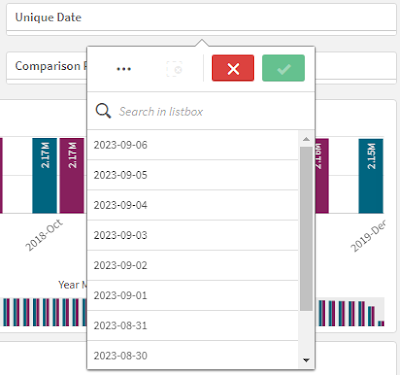
Unique date is a union of all the date representations by granularity of Year, Quarter, Month, Week and Date.

For example,

Year: 2023, 2022, 2021, etc.
Quarter: 2023-Q3, 2023-Q2, etc.
Month: 2023-Sep, 2023-Aug, etc.
Week: 2023-W41, 2023-W40, etc.
Date: 2023-09-09, 2023-09-08, etc.

In this design, it just requires to select the exact date representation directly.  There is no human interpretation and human computation required for the correct  and accurate selection.  In short, what you select is what you get.

Analysis Perspective

Analysis, in general, is always to deal a period.  A period means a start date and an end date in the same granularity level.  There are plenty kinds of representation available (to review), it looks the combination of a date plus the range type is more commonly used.  For example, 2023-09-09 YTD, 2023-06 Rolling 6 Months, etc, i.e. a unique date plus the date range type.  To be more precise, there is a date range type called Actual.  It represents itself.

Analysis perspective also follows strictly on the date integrity.  For example, Unique Date=2023, it does not allow you to select YTD, YTM, Rolling 5 months, etc.  Only if the valid combinations fallen into the same date granularity, it allows the value for selection.  In a lot of traditional design, this is not doing very well.

Comparison Perspective

Comparison is another important element in analysis.  Instead of just looking at the current performance, it also very common to compare the historical performance to see whether it is good or bad.

The most common way to represent comparison is last year, last month, or a specific date.  To make it more generic, it becomes last X Year, last X month or a custom date.  Custom date means any unique date.  It can be Year, Quarter, Month, Week or Date. 

In the implementation, it represents X Years before, X Quarters before, X Months before, X Weeks before and X Days before.  For custom date, it is a list of date representation similar to the Unique date.  Similarly, there is date integrity applied.   For example, if the 2023 Actual, it would not allow the selection of X Months before, X Weeks before because they are not in the valid granularity level.

Front-end Design Improvement

With the capability of the Analytical Calendar, the front-end now can be more neat and clean.  The reason is because there is only two perspectives for periods, i.e. Analysis period and Comparison period.

Analysis period is the period for analysis.  It is similar to the traditional design to select year, quarter, month, week and day.   Comparison period is the period for comparison.  In traditional design it is usually incorporated into the chart and each chart will represent a kind of comparison.

By making use of the Analytical Calendar, all charts now can be possible to provide either or both analysis and comparison period.  There is no need to replicate the same chart to have each to show individual Year, Month or Week, etc for the KPI and the comparison.  All charts are on-the-fly to provide the information based on the user selection.

In other words, it provide a coherent view in terms of usage and experience.  To further let the analysts understand what is being analyzed, on the top left corner, there is a textbox showing both the selection details as well as the actual date range selected.  In this way, it is crystal clear on what analysis is being performed and what comparison is being performed across from the selection to all the charts being shown in the sheet.

Back-end Design Improvement

In order to use the Analytical Calendar, it requires only two variables named vSetAnalysisAnalysisCalendar and vSetAnalysisComparisonCalendar.  The former is used for filtering the Analysis Perspective period while the latter is used for filtering the Comparison Perspective period.

The variable vSetAnalysisAnalysisCalendar is very simple as illustrated below.  It just requires to set the %CONTROL_PERSPECTIVE equals to ANALYSIS and make sure there is no Comparison Perspective.

Similarly, the variable vSetAnalysisComparisonCalendar is also very simple as illustrated below.  It just requires to ignore the %CONTROL_PERSPECTIVE equals to ANALYSIS.

With these two variables, all the expression in the chart development is straightforward.  It just needs to apply the set analysis for the two variables.  

When requiring Analysis Perspective, the below set analysis can be used.

When requiring Comparison Perspective, the below set analysis can be used.

As the front-end is now consistent and coherent, the same expression can be applied and across all the charts.  Unless, there are specific chart would be shown, these two kinds of expressions can satisfy a majority of the use cases.  Definitely, the Analytical Calendar can also be applied to more advanced use scenarios which would not cover here.

Other Advantages

Indeed, the Analytical Calendar also has other advantages.  In designing the data model, majority of the time would fall into a situation to pre-build a data or to calculate on the fly.  The rule of thumb is always to pre-build it if possible to minimize the computation required during use.

When manipulating date, there are also a few scenarios that might not be generic for every usage.  For example, if today is 2023-09-09, should it allow the selection of 2023-Sep?  In my experience, it depends on the flavor of the end users but this becomes a question of developers for a proper expression development.  Another example is the cross year week.  There are different ways to handle the incomplete week like making it full week and count as the previous year week or the let the week to be incomplete.  This is a headache not just to developer but also the analysts using the interactive dashboards.

Thus, the design of Analytical Calendar also incorporates this element.  It allows to pre-calculate all these into the data model and do not need very complicated on-the-fly expression to calculate the results.  It can still maintain as Analysis Perspective and Comparison Perspective.  The below are some scenarios for sharing.

This concludes how to use the Analytical Calendar.  Please leave me message if further discussion is needed.

Thank you for reading.  I hope it help you.  Just leave a message if you have any discussion/share want to make.